ML Foundations: Support Vector Machines (SVMs)

ML Foundations: Support Vector Machines (SVMs)

Introduction

In our machine learning series, we’ve explored models that classify data in different ways. Logistic Regression finds a line that separates classes based on probabilities. Decision Trees use a series of if/else questions. Now, we turn to another powerful and elegant classification algorithm: the Support Vector Machine (SVM).

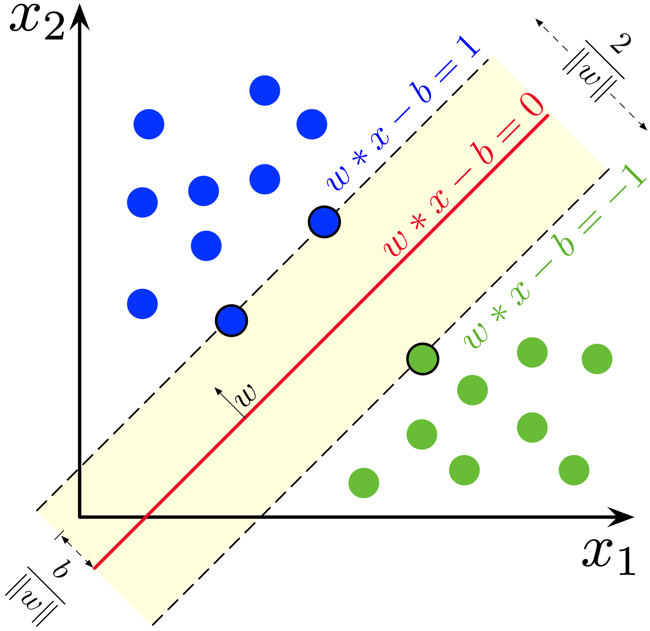
The core idea behind SVMs is to find the best possible dividing line (or hyperplane) that separates two classes. But what does “best” mean? For an SVM, it means finding the line that is as far away as possible from the nearest data points of each class. This gap is called the margin, and SVMs are all about maximizing it.

This focus on the margin makes SVMs a “large margin” classifier, which often leads to high accuracy and good generalization to new data.

In this guide, we’ll build an intuition for:

1. The concept of the margin and why maximizing it is a good idea.
2. Support Vectors: The critical data points that define the decision boundary.
3. How SVMs handle outliers with soft margin classification.
4. The Kernel Trick: The magic that allows SVMs to model complex, non-linear relationships.

1. The Intuition: Maximizing the Street

Imagine your data points are two groups of houses on a map, and you want to draw a straight road that separates them. You could draw many possible roads. Which one is best?

An SVM’s approach is to find the road that is as wide as possible—one where the “lanes” on either side, which touch the nearest houses, are maximized. The road itself is the decision boundary, and the edges of the lanes are defined by the closest data points.

This “widest street” approach is powerful because it creates a decision boundary that is robust. It’s less sensitive to the exact location of most data points and is determined only by the most extreme points—the ones closest to the other class.

2. Support Vectors: The Critical Few

Those data points that lie on the edge of the “street” or margin are called support vectors. They are the most important data points in the dataset because they alone support or define the decision boundary.

If you were to move any of the other data points (the ones not on the margin), the decision boundary wouldn’t change. But if you move a support vector, the boundary will shift. This is a key insight: SVMs are highly efficient because their decision function is defined by only a small subset of the training data.

This is called hard margin classification. It works beautifully if the data is perfectly linearly separable, but it has two major problems in the real world:

1. It only works if the data is perfectly separable.
2. It is extremely sensitive to outliers. A single outlier can dramatically change the decision boundary.

3. Dealing with the Real World: Soft Margin Classification

To create a more flexible and robust model, we can soften the margin. Soft margin classification allows for a trade-off between maximizing the margin and allowing some data points to be on the wrong side of the margin (or even on the wrong side of the decision boundary).

We control this trade-off with a hyperparameter, often denoted as C.

• Low C value: Creates a wide margin. The model is more tolerant of margin violations. This leads to better generalization but potentially less accuracy on the training set.
• High C value: Creates a narrow margin. The model tries to fit the training data as perfectly as possible, allowing very few margin violations. This can lead to overfitting if C is too high.

In Scikit-Learn, C is a regularization parameter. It’s the inverse of the regularization strength: smaller C means stronger regularization.

4. The Magic of Non-Linearity: The Kernel Trick

So far, we’ve only talked about linear decision boundaries. But what if your data isn’t separable by a straight line?

This is where SVMs truly shine. They can model complex, non-linear boundaries using a mathematical technique called the kernel trick.

Here’s the intuition:

1. The SVM projects the data into a higher-dimensional space where it is linearly separable.
2. It then finds a linear decision boundary (a hyperplane) in that higher-dimensional space.
3. When this hyperplane is projected back down to the original, lower-dimensional space, it appears as a complex, non-linear boundary.

Imagine a 1D line of data with alternating red and blue points. You can’t separate them with a single point. But if you project them into 2D by, for example, squaring the values (y = x²), they become a parabola, and you can easily separate them with a horizontal line.

The “trick” is that SVMs don’t actually perform this transformation, which would be computationally very expensive. Instead, kernel functions can compute the result of the dot product between two vectors as if they had been projected into a higher-dimensional space, without ever creating those new features.

Common kernels include:

• Polynomial Kernel: Can model curved decision boundaries.
• Radial Basis Function (RBF) Kernel: Can create complex, circular, or blob-like boundaries. This is the most popular and powerful kernel.

5. Practical Example with Scikit-Learn

Let’s use Scikit-Learn to see a linear SVM and an RBF kernel SVM in action.

import numpy as np
import matplotlib.pyplot as plt
from sklearn import datasets
from sklearn.model_selection import train_test_split
from sklearn.preprocessing import StandardScaler
from sklearn.svm import SVC
from sklearn.metrics import accuracy_score

# Generate some data that is not linearly separable
X, y = datasets.make_moons(n_samples=100, noise=0.15, random_state=42)

# Split and scale the data
X_train, X_test, y_train, y_test = train_test_split(X, y, test_size=0.3, random_state=42)
scaler = StandardScaler()
X_train_scaled = scaler.fit_transform(X_train)
X_test_scaled = scaler.transform(X_test)

# --- 1. Train a Linear SVM ---
# This will try to find a straight line to separate the "moons"
linear_svm = SVC(kernel='linear', C=1.0, random_state=42)
linear_svm.fit(X_train_scaled, y_train)
y_pred_linear = linear_svm.predict(X_test_scaled)
print(f"Linear SVM Accuracy: {accuracy_score(y_test, y_pred_linear):.3f}")

# --- 2. Train an SVM with an RBF Kernel ---
# This can model a non-linear boundary
rbf_svm = SVC(kernel='rbf', C=1.0, gamma='auto', random_state=42)
rbf_svm.fit(X_train_scaled, y_train)
y_pred_rbf = rbf_svm.predict(X_test_scaled)
print(f"RBF Kernel SVM Accuracy: {accuracy_score(y_test, y_pred_rbf):.3f}")

You will see that the RBF Kernel SVM achieves much higher accuracy because it can create a decision boundary that correctly follows the curved shape of the moons dataset.

Conclusion

Support Vector Machines are a powerful and versatile class of models. They offer a unique perspective on classification by focusing on maximizing the margin between classes.

• Key Idea: Find the decision boundary that is as far as possible from the nearest data points of each class.
• Support Vectors: The few, critical data points that define this boundary.
• Soft Margin (C parameter): Provides a way to handle real-world, messy data by trading off margin width for misclassifications.
• The Kernel Trick: The “magic” that allows SVMs to efficiently model highly complex, non-linear decision boundaries without explicitly creating higher-dimensional features.

While deep learning has become dominant in areas like image and text processing, SVMs remain a go-to algorithm for small-to-medium-sized tabular datasets, often delivering excellent performance with careful tuning.

Suggested Reading

• “An Introduction to Statistical Learning” by James, Witten, Hastie, and Tibshirani: Chapter 9 provides a clear and detailed explanation of SVMs.
• StatQuest with Josh Starmer on YouTube: His video on SVMs is an excellent visual introduction to the concepts of margins and kernels.
• Scikit-Learn Documentation: The user guide on SVMs provides many examples and details on the different kernels and parameters.